Final çalışması – Çözüm 1

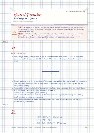
Not always. when an entire row in Routh table becomes zero, it means that at least two poles are on the imaginary axis OR real axis OR complex poles symmetric with respect to the origin

Steady state error is due to the type of the system as well as the input signal. For example a type 1 system can follow an step input while inputs like ramp or parabolic signals are not followed accurately.

No, stability is a characteristic of the system itself and does not depend on the input signal.

Pole placement: reduces stability, increases accuracy

increases the settling time (slow response)

Zero placement: Increases stability, faster responses will appear (decreasing the settling time), can lead to noise augmentation

In terms of performance, when poles are added, max. overshoot is reduced but for zero placement, M_p% increases.

The steady state error is 10%

So the second condition may not be satisfied, and for any value of k_2 , the system tracks unit step input!

So in order to have no change in sign, all components of the first column must be positive, which gives the following conditions,

from the above two conditions we find out that k must be positive (greater than zero).

Now let's check the last condition.

So in total the acceptable range is 0<k<1.395 5%

unmatched branches : n-m=3 ⇒ 3 asymptotes

the centroid of asymptotes may be determined as

Now, let's calculate the breaking points by using the characteristic equation

The first two roots are on the root locus, so they are accepted as break out and break in points.

Now let's determine the angles of leaving from the complex poles,

we can also determine the intersection of the root locus with the imaginary axis by using the Routh table as,

There are two cases where we can construct a full zero row, in the s^1 row. For k=38.68 and k=116.31 this row becomes zero, the auxiliary equation for these two cases are

So the jω -crossings are 5%

According to the current data, we can plot the root locus to a high degree of accuracy, but if we want explicit and analytical definition for various branches we should check the phase condition by substituting s=σ+jω in the open-loop transfer function.

for positive feedback, the root locus plot is